Designing Coaxial Connectors with CST Studio Suite

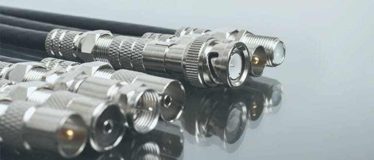
In this blog post we’ll take a look at the analysis and simulation of coaxial high-frequency connectors with CST Studio Suite. These connectors are suitable for the high requirements of 5G networks. They have applications in radio, video and audio technology and in laboratory use for oscilloscopes and measuring devices. These connectors are also commonly used in data systems and telecommunications applications.

Image 1: Coaxial connectors in radio technology
Image 2: Coaxial connectors in laboratory use

A connector consists of two conductors: the inner and outer conductors. Between the conductors there is either the insulator or the air as a dielectric.

Function and Properties of Coaxial Connectors

Coaxial connectors allow detachable connection of coaxial cables. Assembly and installation are simple, while electromagnetic interference and radiation are low.  Coaxial connectors are manufactured with good electrical shielding. They are often produced with a 50 Ω or a 75 Ω characteristic impedance and have excellent return loss.

Various forms of coaxial connectors:
Fig. 3: SMA adapter
Fig. 4: Hand attaching/removing antenna jack
Fig. 5: Lan wire with connector RJ 45

Manufacturer data sheets list key coaxial connector specifications such as power transfer, return loss, frequency range, characteristic impedance, and passive intermodulation.

Important Parameters for the Evaluation of the Connectors

Characteristic Impedance and Impedance Matching

An important parameter of a coaxial connector is the characteristic impedance along the connector. The characteristic impedance, or the impedance of the connector, Z, is independent of the line length and the signal frequency. The unit is ohms. Connectors with a characteristic impedance of 50 Ω (general RF technology) or 75 Ω (television technology) are common, rarely 60 Ω (old systems) or 93 Ω. The value can be determined experimentally using time domain reflectometry. The characteristic impedance is calculated from the ratio of the inner diameter D of the outer conductor and the diameter d of the inner conductor of the connector and the dielectric properties (relative permittivity εr) of the insulation material (dielectric):

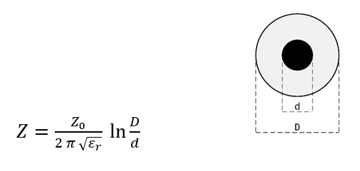
Figure 6: with the characteristic impedance of the vacuum

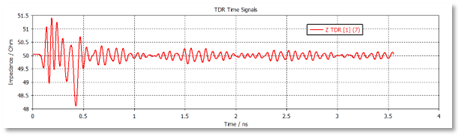
Figure 7: Impedance matching: 50 Ω along the connector

The power that can be transmitted through a coaxial cable depends on the characteristic impedance. At a characteristic impedance of 30 Ω, the transmittable power is maximum.

Depending on the application, the characteristic impedance is therefore selected.

• TV and radio technology: 75 Ω to keep losses low.
• Communication technology: 50 Ω to have good transmission characteristics in both receiving and transmitting. (Average value between 30 Ω and 75 Ω).

Reflection, Line Matching and Return Loss

Coaxial cables for high-frequency applications are generally operated in line matching. The load resistance of the cable should match the characteristic impedance as closely as possible so that no reflections occur at the end of the line, which can cause standing waves and increased losses. The degree of mismatch is determined using time domain reflectometry. To assess the mismatch, the value of return loss is measured. Return loss is the ratio of reflected power in source or port 1 to forward power in port 1 on a logarithmic scale, S₁₁.

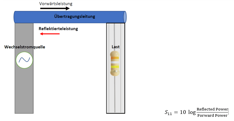
Figure 8: Forward and reflected power

Reflections occur at all points where the characteristic impedance changes, even with unsuitable connectors at higher frequencies. Any change in the inner and outer diameter and any change in material along a connector will cause the characteristic impedance to change. These discontinuity positions in the length of a connector cause the generation of the standing wave and finally the reflection coefficient increases.

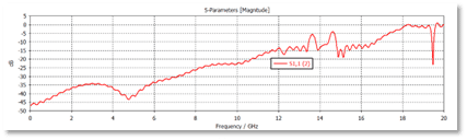
Figure 9: reflected power or return loss, S₁₁.

Modeling and the Base Model

The development of a high-frequency connector requires a base model in order to make changes and optimizations. Usually, this 3D base model is available in-house. CST Studio Suite’s ability to import different types of 3D CAD models gives development teams great flexibility. CATIA, SOLIDWORKS, Abaqus, Nastran and Step files, to name a few, are 3D models supported by CST for data import and export.

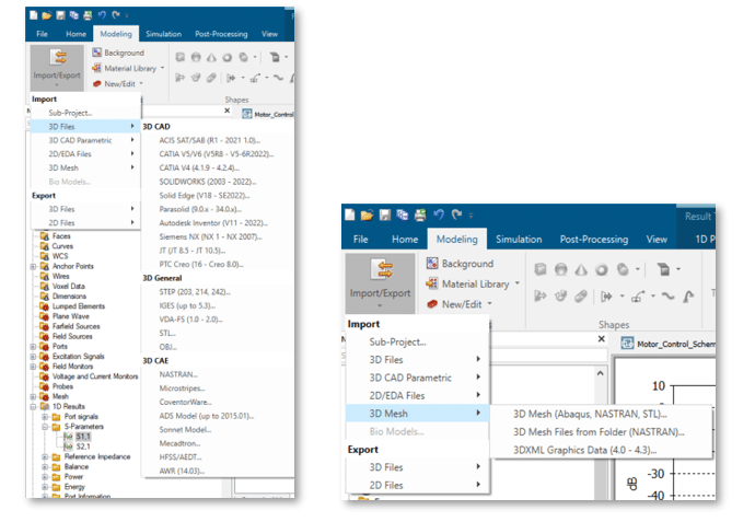
Figure 10: Different types of 3D CAD models available in CST Studio Suite

In addition to 3D model import and export, the CST Studio Suite library includes a diverse collection of examples compiled for different electromagnetic and mechanical simulation requirements. For our example, a 3D model of a 90 degree angle connector was selected from the CST Studio library.

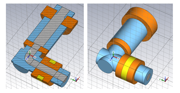
Figure 11: 3D model of a 90 degree angle connector from the library of the CST Studio Suite

Electromagnetic Simulation with CST Studio Suite

Quick Check: Simulation of the Base Model

For the simulation of the base model it is necessary to make the simulation setting first. This means that all materials with the corresponding electromagnetic properties are defined and the boundaries of the simulation environment are set. In addition, the physical properties of the simulation domain are determined. As a last step, the bandwidth of the simulation is defined and the appropriate CST solver is selected.

The simulation result of the base model shows a deviation of more than 5 Ω from the standard 50 Ω. At the highlighted point in the diagram below, it is 45 Ω, which is outside the tolerance range. At the end of the connector, the value is 51 Ω instead of 50 Ω, which is also undesirable.

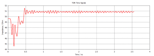
Figure 12: The TDR simulation result of the base model

As a result, design improvement is essential for industrial applications. Simulation and optimization are necessary for this.

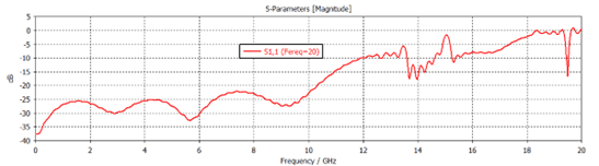
Figure 13: The return loss of the basic model

The return loss result also highlights that the reflection is not optimal and optimization is required for a product that meets the requirements.

Parameterization of the Model

The simulation in the last section showed the need for improvement of the basic model to meet the requirements of an industrial connector. Any improvement is made by changing either the geometric dimensions or the electrical properties of the components. For this purpose, the system is parameterized with respect to both the size and the physical properties of the components. Parameterization allows optimization of the model or material and gives the development teams a high degree of flexibility in the simulation. In the example, 15 different physical quantities were parameterized. Two of them are shown as examples in the following figure.

Figure 14: Parameterization of physical quantities in CST Studio Suite

Sensitivity Analysis of the Model

After parameterization, the critical dimensions of the system can be found through a considered parameter change. At the same time, it is important to understand in which direction a parameter must be changed to make the connector work better. With the sweep function of the CST Studio Suite it is possible to observe the results of the simulation for a combination of parameter changes.

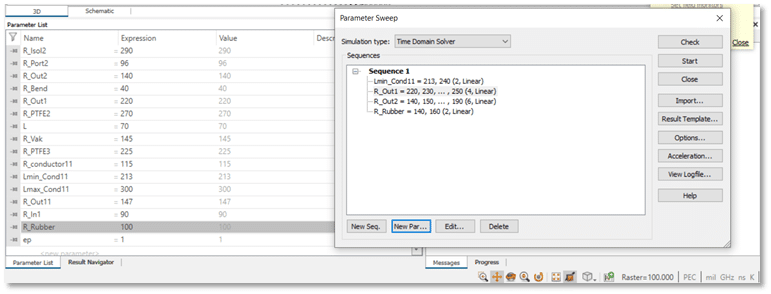
Figure 15: Sensitivity analysis of the model

The following impedance curve along the connector is obtained after using the CST sweep function for four parameters. An improvement of more than 3.5 Ω compared to the base model is achieved after simulation and parameter changes.

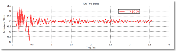
Figure 16: Impedance curve along the connector after sensitivity analysis

The CST Studio Suite offers the possibility to monitor all electromagnetic properties of the system. The electric and magnetic fields are displayed in different frequencies.

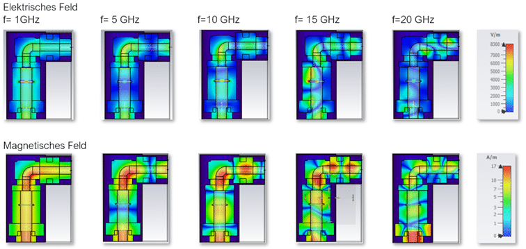
Figure 17: Electric and magnetic fields in different frequencies

Optimization of the Model

The results of the sensitivity analysis can be used as a basis for further improvements with the help of the CST Studio Suite Optimizer. The optimizer offers the possibility to calculate the best results using different artificial intelligence algorithms. In the first step, the appropriate algorithms and the parameters that will be changed are selected. The parameters used here are the crucial parameters obtained from the sensitivity analysis.

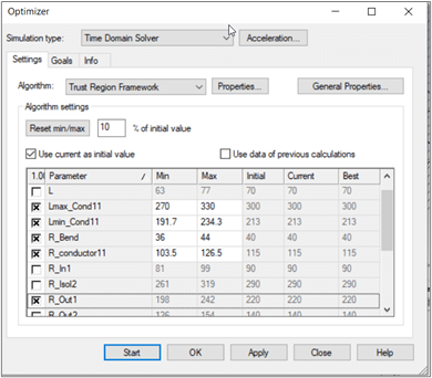
Figure 18: Optimization of the model with CST Studio Suite

Then, in the second step, the target functions are defined. For example, the target values of the return loss are defined for different bandwidths.

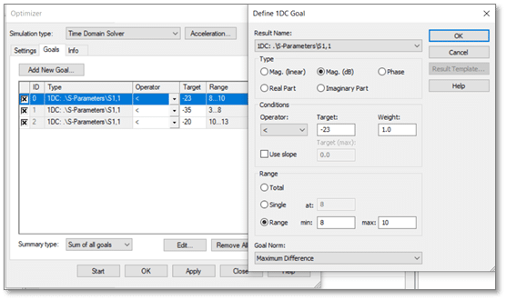
Figure 19: Definition of the objective functions in CST Optimizer

The simulated results of the base model, sensitivity analysis, and CST optimization are compared in the following diagram.

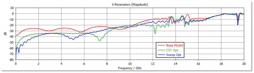
Fig. 20: Comparison of the return loss values

The desired improvement after optimization is shown in the following table.

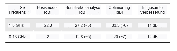
Fig. 21: Improvement in return loss after optimization

Thermal Simulation

To develop a high-performance connector, an electromagnetic design is usually not enough. At high power levels, the temperature of the components can be very high, and it must be ensured that these temperatures are not greater than the permissible values. For this purpose, CST Studio Suite offers electromagnetic-thermal coupling simulation. In such simulations all electrical and magnetic volume losses as well as surface losses, are transferred to the thermal simulation as a heat exciting source.

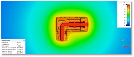
Figure 22: Power= 40 W; Tmax= 50.4˚C

Figure 23: Power= 20 W; Tmax= 35.2˚C

Shown here are the results for 20 watts and 40 watts of power. If the temperature is above the accepted value, either the electromagnetic design must be changed, or a cooling system must be included in the connector design.

Summary

A connector that was not suitable for industrial applications was optimized using CST Studio Suite. During the optimization, changes in the geometry resulted in a significant improvement in the connector’s electromagnetic properties. The wave impedance along the connector is now close to the desired 50 Ω and the return loss is about 12 dB lower than before the design optimization.

The advantages of an electromagnetic simulation with CST Studio Suite can be summarized in the following important points:

• Significantly improved electromagnetic properties
• Optimize device performance
• Detailed insights into product features
• Shorter development times using optimization tools
• Reducing the number of initial prototypes and physical tests
• Lower costs